Home | Abstract | Intro | Page 1 | Page 2 | Results | Conclusions | References | Acknowledgements

HEC-HMS Analysis 

HEC-HMS requires the area, input losses, rate transformation and baseflow for each watershed:

• Area of Watershed
  • input was in square miles
    
• Input Losses
  • Initial loss was 0 inches, to allow maximum runoff
  • Percent impervious was 0 - this is a natural watershed, with an assumption of no impervious surfaces
  • A curve number of 65 was used
    
• Rate Transformation
  • Calculated SCS Lag times were used for each watershed
    
• Baseflow
  • An assumption of no baseflow was designated because flow doesn’t occur in the ditch during dry periods.  The HEC-HMS model suggests that in this case, the lake component be modeled as a "sink".

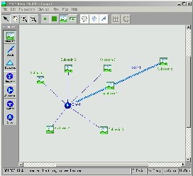
The HEC-HMS simulations were run using 2 scenarios – the first using only the area from Basin 1 and a second simulation including areas from both Basins 1 and 2.  Adding the area from Basin 2 assumes that all flow from that basin is captured by the ditch, and diverted into the lake.

Figure J - HEC-HMS Model of Stoneman Lake Basin 1

Figure K - HEC-HMS Model of Stoneman Lake Basins 1 and 2

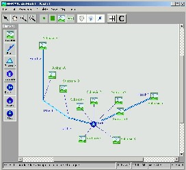
It must be noted that HEC-HMS will not allow one sub-basin to flow into another.  To compensate for this limitation, Reaches 1 and 2 will delay flow into the lake.  A lag time for each reach is determined by the sub-basin it theoretically flows into.  Reach 1 has a lag of 5.11 minutes – the same as Sub-basin 4.  Reach 2 has a lag of 18.58 minutes – the same as Sub-basin 8.  This adaptation will generate a more correct peak flow time for the lake (sink). 

Meteorological Models were based on 2-year, 50-year, and 100-year storms with a 24-hour duration for this area of Arizona¹¹ (see Table 7).  A Type II SCS Hypothetical rainfall model was selected for each simulation.

 Table 7 - Event Storm Precipitation 

A 5-minute interval was used as a time step to calculate the runoff hydrograph.  A theoretical 24 Hour storm started on December 16, 2002 at 12:00 Noon (the choice of this date was purely arbitrary).

Precipitation

In addition to watershed delineation, I placed 2 rain gages on each of the two main watersheds to measure precipitation.  I collected rainfall from July – December 2002, and precipitation totals are listed in Table 8.  The locations of these gages are shown in Figure L:

Figure L – Gage Locations

Measurements were taken using a tipping bucket rain gage (see Figure M).  When downloading data from a Hobo Event Logger, I took an average of the volume each bucket was recording at the time.  Each rain gage was recalibrated at this time so that each bucket would collect equal volumes of water.  After a period of about two weeks, each bucket would be different from the other by about .5 milliliters, or 5%.

Figure M – Tipping Bucket Rain Gages

Gages had a +/- 5% error in measurement.

Converting volume recorded from ml to inches of rainfall requires a calibration factor.  The calibration factor accounts for an 8" diameter area of the gage.  The 8" diameter of the gage = 50.27 in² of catch area.   Inches of rainfall is calculated by converting from milliliters:

Calibration Factor x Number of Tips = Inches Rainfall

Example:

If the logger registered 75 tips on October 1, then:
75 tips x 0.01214 in / tip = 0.91 inches of rain fell on October 1.

In addition to collecting precipitation data at Stoneman Lake, additional precipitation data was downloaded from the National Climatic Data Center¹² in order to compare values between Stoneman Lake and adjacent stations.  Happy Jack Ranger Station and Flagstaff Airport data was compared to rainfall recorded at Stoneman Lake.  A percent difference was calculated to show differences between the stations.

 Table 9 – Precipitation Values of Three Local Stations, 2002 

*July data is incomplete due to a tipping bucket getting stuck, and not recording data for a period of 2 weeks.

A comparison graph of precipitation data is shown in Figure N.  Using rainfall data from multiple stations may allow a correlation ratio between rainfall in adjacent watersheds. In the future when my gages will no longer exist, this might help in potential analysis of the basin.

Home | Abstract | Intro | Page 1 | Page 2 | Results | Conclusions | References | Acknowledgements